Steady-State Examples

Steady-state Dyson equation: Anderson Impurity model

Synopsis

We first demonstrate the use of the steady-state implementation for a perturbative solution of transport through a single impurity Anderson model. The on-site impurity Hamiltonian is

\[H_{loc} = U n_\uparrow n_\downarrow + \left(\mu-\frac{U}{2} + \epsilon_d\right)(n_\uparrow + n_\downarrow),\]

where \(U\) is the local interaction, and \(\epsilon_d\) the bare level energy; \(\mu=0\) will be set to zero in the following, such that \(\epsilon_d=0\) corresponds to a particle-hole symmetric case. The impurity is coupled to two infinite metallic leads, the left (\(L\)) and right (\(R\)) bath, which are kept at a voltage bias \(V\). Integrating out the leads gives rise to an embedding self-energy \(\Sigma_{\rm bath}=\Sigma_{L}+\Sigma_{R}\), which is defined via a spectral representation. We use a smooth box density of states

\[A_\Sigma(\omega) = \frac{\Gamma/\pi}{(1+e^{\nu(\omega-\omega_c)})(1+e^{-\nu(\omega_c+\omega)})},\]

where \(\Gamma\) is the hybridisation strength, \(\omega_c\) is the half bandwidth, and \(\nu\) a smoothening parameter. While the density of states \(A_\Sigma(\omega)\) is identical for the left and right baths, \(\Sigma^<_{L,R}\) is given by the equilibrium distribution with different chemical potentials \(\mu_{L/R}=\pm V/2\). In the following, we use \(\omega_c=10\Gamma\) and \(\nu=3/\Gamma\); \(\Gamma=1\) defines the energy unit, and \(1/\Gamma\) is the unit of time.

The noninteracting impurity Green’s function \(G_{0}\) is therefore determined through the steady-state variant of the Dyson equation \(G_0 =( i\partial_t + \mu - \Sigma_{\rm bath})^{-1}\), while the interacting Green’s function \(G\) is obtained from a Dyson equation \(G =( i\partial_t + \mu - \Sigma_{\rm bath}+\Sigma_U)^{-1}\), with an additional self-energy \(\Sigma_U\) due to interactions. In the example below, we approximate \(\Sigma_U\) by a (non self-consistent) 2nd order perturbation theory, i.e., \(\Sigma_U\) is given by

\[\Sigma(t,t') = U(t) G_0(t,t') G_0(t,t') G_0(t',t) U(t'),\]

evaluated in the steady state.

Finally, the current is defined by the rate of particle transfer from the left to the right reservoir, \(J= \frac{dN_L}{dt}= -\frac{dN_R}{dt}\). An exact expression can be derived using equations of motion for the Green’s functions, and is given by equal-time convolution

\[J = 2\left(\Sigma_L\ast G - G\ast\Sigma_L\right)^<(t,t),\]

where the factor \(2\) is due to spin. This relation is in general not satisfied away from half-filling in bare (non-conserving) second order perturbation theory. In the steady state, the current can be evaluated using the convolution_density_matrix method, see Integral transforms,

\[J = -2i\left( \rho_{\Sigma_L,G} - \rho_{G,\Sigma_L} \right) =4\text{Im} \left( \rho_{\Sigma_L,G} \right).\]

Here the second equation uses hermitian symmetry \(\rho_{\Sigma_L,G} = \rho_{G,\Sigma_L}^\dagger\).

Details and Implementation

The relevant files for the implementation, found in nessi/examples/, are listed in the table below.

programs/ness2_siam.cpp	Source code.
utils/demo_ness2_siam.ipynb	Jupyter notebook to run the program.
utils/demo_ness2_siam.py	A Python script; same as the notebook.

The implementation is built on the functions in the ness2 namespace. The input parameters for the main program are the physical parameters U (interaction \(U\)), beta (inverse temperature \(\beta\)), V (voltage bias \(V\)), and epsd (on-site energy \(\epsilon_d\)), as well as the numerical parameters Nft (number of time/frequency points) and h (timestep \(h\)). Moreover, we allow for a nonzero eta for the regularization of the Dyson equation (which can however be set to zero in the example below, and would only be relevant if the level \(\epsilon_d\) has no spectral overlap with the baths). After reading the input parameters from the input file we initialize herm_matrix_ness objects

herm_matrix_ness G0(Nft,size);

for the noninteracting Green’s functions \(G_0\), and similar for G (\(G\)), SL (\(\Sigma_L\)), SR (\(\Sigma_R\)), Sbath (\(\Sigma_L+\Sigma_R\)), SU (\(\Sigma_U\)), and S (\(\Sigma_L+\Sigma_R+\Sigma_U\)). Next, the left and right baths are initialized with the given smooth box density of states. For this, we define a class to provide the density of states.

class box_dos{
public:
  double hi_,lo_,wc_,nu_;
  box_dos() wc_(10.0), nu_(3.0), hi_(15.0), lo_(-15.0) {}
  double operator()(double w){
    return 1/((1+exp(nu_*(w-wc_))*(1+exp(-nu_*(wc_+w)));
  }
};

Here hi_ and lo_ define the bounds of the integrals in the spectral representation. The bath self-energies are then initialized using

box_dos dos();
green_equilibrium_ness(FERMION,SL,dos,beta,+0.5*V,h,FFT_TRAPEZ);
green_equilibrium_ness(FERMION,SR,dos,beta,-0.5*V,h,FFT_TRAPEZ);
Sbath=SL;
Sbath.incr(SR,1.0,fft_domain::time); // Sbath+= SR on time-data

Next we solve the noninteracting Dyson equation using

cdmatrix eps_matrix(1,1);
eps_matrix(0,0) = epsd;
dyson(G0,mu,eps_matrix,Sbath,h,FFT_TRAPEZ,BATH_GAUSS,eta,beta,mu);

Here we allow for the regularization using the gaussian bath if eta is nonzero. With the resulting G0 one can determine the 2nd order self-energy. The structure of the diagram is analogous as for the previous real-time example, and hence also the implementation is similar:

herm_matrix_ness W(Nft, size1);  // temporary W
Bubble1_ness(W, G0, G0);  //W(t,t') <- ii*G(t,t')G(t',t)
W.smul(U*U,fft_domain::time); // W(t,t') <- U^2 W(t,t')
Bubble2_ness(SU,G,W); //Sigma_U(t,t')<-ii*G(t,t')W(t',t)
SU.smul(-1.0,fft_domain::time);

Finally, we solve the interacting Dyson equation:

S=Sbath;
S.incr(SU,1.0,fft_domain::time); // S += SU
dyson(G,mu,eps_matrix,S,h,FFT_TRAPEZ,BATH_GAUSS,eta,beta,0);

For postprocessing we compute the convolutions

cdmatrix SUG,SLG,rho;
convolution_density_matrix(SLG,FERMION,SL,G,h); // ii*[SL*G]^<(t=0)
convolution_density_matrix(SUG,FERMION,SU,G,h); // ii*[SU*G]^<(t=0)
density_matrix(rho,FERMION,G); //   = ii*G^<(t=0)
double Current = 4.0*SLG.trace().imag();
double Eint = (SUG).trace().real(); // interaction energy
double dens = 2*rho.trace().real(); // <n_up + n_do >

Finally we update the frequency-domain Green’s functions, such that we can later analyze the spectra:

G.transform_to_freq(h,FFT_TRAPEZ);

At the end, all output is stored into a single HDF5 file:

// create the hdf5 file (char *flout points to the filename)
hid_t file_id = open_hdf5_file(flout);
// write Nft to group "/Nft" in the file :
store_int_attribute_to_hid(file_id, "Nft", Nft);
[...] // similar for dens, Eint, Current
G0.write_to_hdf5(file_id, "G0"); // new group "/G0" in file
[...]  // same for G,S,...
close_hdf5_file(file_id);

The HDF5 output is conveniently interpreted using the Python utilities provided with the ReadNESS modules.

Discussion

Fig. 18 c) shows converged results for the interacting impurity spectral functions \(A(\omega)\) and the noninteracting impurity spectral functions \(A_0(\omega)\), for a given bath as shown in Fig. 18 a). The spectrum is essentially a Lorentzian peak, which becomes slightly more broadened for nonzero interaction \(U\). The non-equilibrium nature of the state is evident from the distribution function

\[F(\omega) = \frac{G^<(\omega)}{2\pi i A(\omega)}.\]

The latter becomes clearly non-thermal, simultaneously reflecting the Fermi edges in the left and right bath (see Fig. 18 d)). Interactions support thermalization and therefore slightly reduce the sharp edges, compare the blue and red curves in Fig. 18 d) for \(F(\omega)=G^<(\omega)/2\pi i A(\omega)\) and \(F_0(\omega)=G_0^<(\omega)/2\pi i A_0(\omega)\), respectively.

Fig. 18 b) shows the current as a function of the voltage, which evolves from the linear response regime at small \(V\) to a saturated value of \(J=2\) (corresponding one transport channel for each spin) when \(V\) becomes comparable to bandwidth \(2\omega_c\), such that the left (right) bath is full (empty). In the interacting case, the current is reduced, consistent with the broadening of the steps in the distribution function. Of course, the bare second order perturbation theory cannot correctly describe the Kondo effect at low temperatures and large \(U\), which is not in the scope of the present code. The steady state code can however be easily combined with a more accurate diagrammatic computation of real-time Green’s functions and self-energies in the steady state.

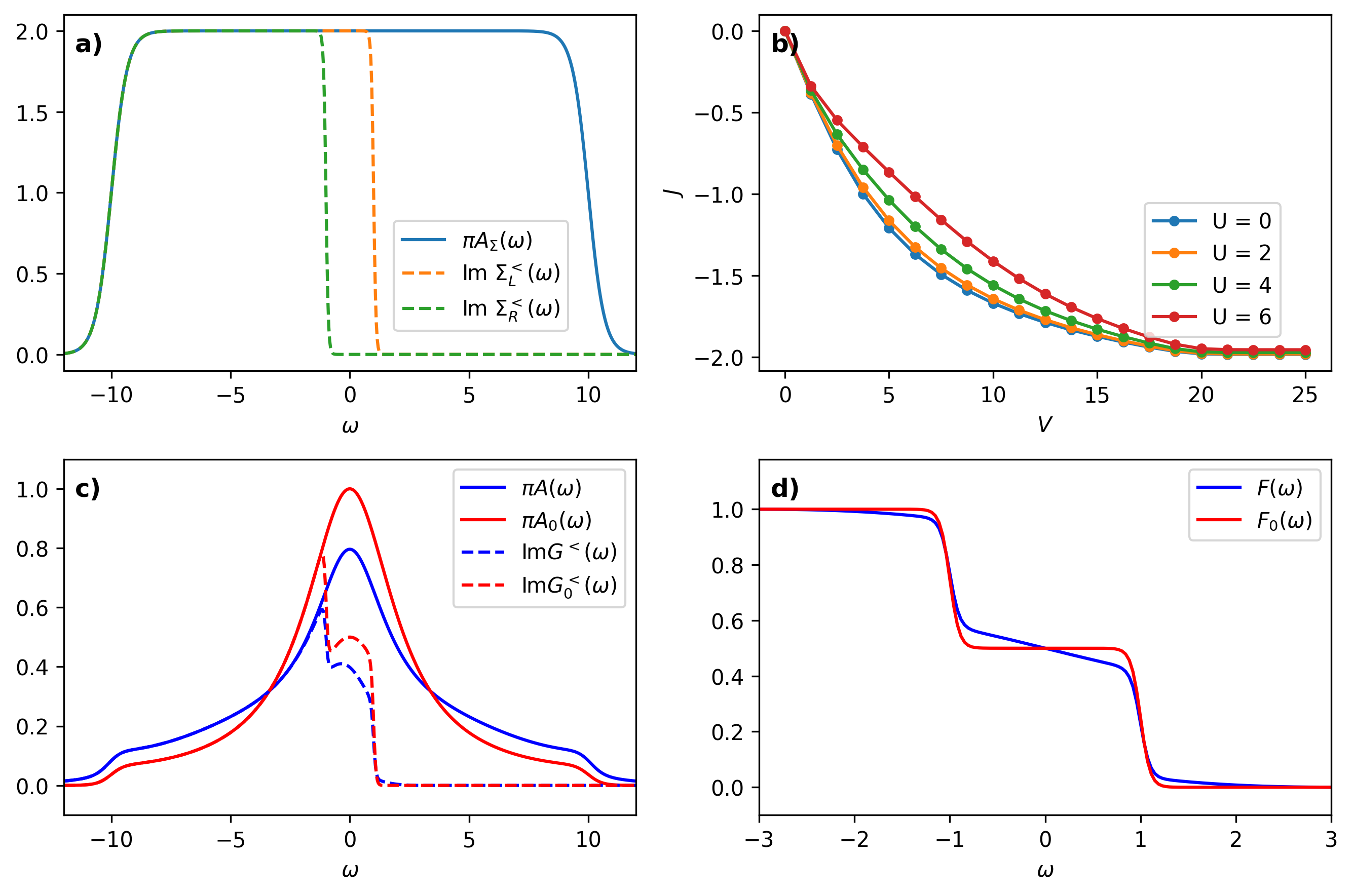
Fig. 18 Results for the Anderson model. Anderson model for \(U=6\), and \(\beta=20\). a) Bath spectral functions and occupation functions (dashed) for voltage \(V=2\). b) Current as function of voltage \(V\), for \(\beta=20\). c) Interacting spectral function \(A(\omega)\) (full blue lines) and noninteracting spectral function \(A_0(\omega)\) (full red lines) for \(V=2\). The dashed lines show the imaginary part of the corresponding lesser Green’s functions. d) Occupation functions for the interacting case (\(F(\omega)\)) and noninteracting case (\(F_0(\omega)\)) for \(V=2\).

In Fig. 19, we demonstrate the numerical convergence of the steady state approach (for \(U=6\), \(V=2\), \(\beta=20\)). We first fix a small value \(h=0.001\) of the timestep, and perform simulations with different length \(N_{\rm ft}\) of the Fourier domain. This tests the convergence with the maximal real time \(t_{\rm c}= h N_{\rm ft}/2\) which is represented by the time grid. For accurate results, it is necessary that all functions \(G^{R,<}(t)\) and \(\Sigma^{R,<}(t)\) essentially decay to zero within the domain \(|t|<t_{\rm max}\). In Fig. 19 a), we plot the difference \(|J(N_{\rm ft}) - J_{\rm ref}|\), where the reference result \(J_{\rm ref}\) is simply the result for the largest grid (\(N_{\rm ft}=2^{20}\)). The sharp drop in the error \(|J(N_{\rm ft}) - J_{\rm ref}|\) is consistent with an exponential decay of \(|G^{R,<}(t)|\) and \(|\Sigma^{R,<}(t)|\), such that there is no dependence on \(t_{\rm c}\) for sufficiently large \(t_{\rm c}\).

To analyze the convergence with the timestep \(h\), we perform simulations with different \(N_{\rm ft}\) and \(h\), keeping the product \(N_{\rm ft}h\) fixed. This corresponds to varying \(h\) at fixed cutoff \(t_c\); the latter is chosen as the largest value in Fig. 19 a), i.e., \(hN_{\rm ft} = 0.001 \times 2^{20}\). The error \(|J(N_{\rm ft}) - J_{\rm ref}|\) with respect to the reference result \(J_{\rm ref}\) at the largest \(N_{\rm ft}\) (smallest \(h\)) is shown in Fig. 19 b). The plot demonstrates an error of order \(\mathcal{O}(h^2)\), consistent with the trapezoidal evaluation of the convolution integrals.

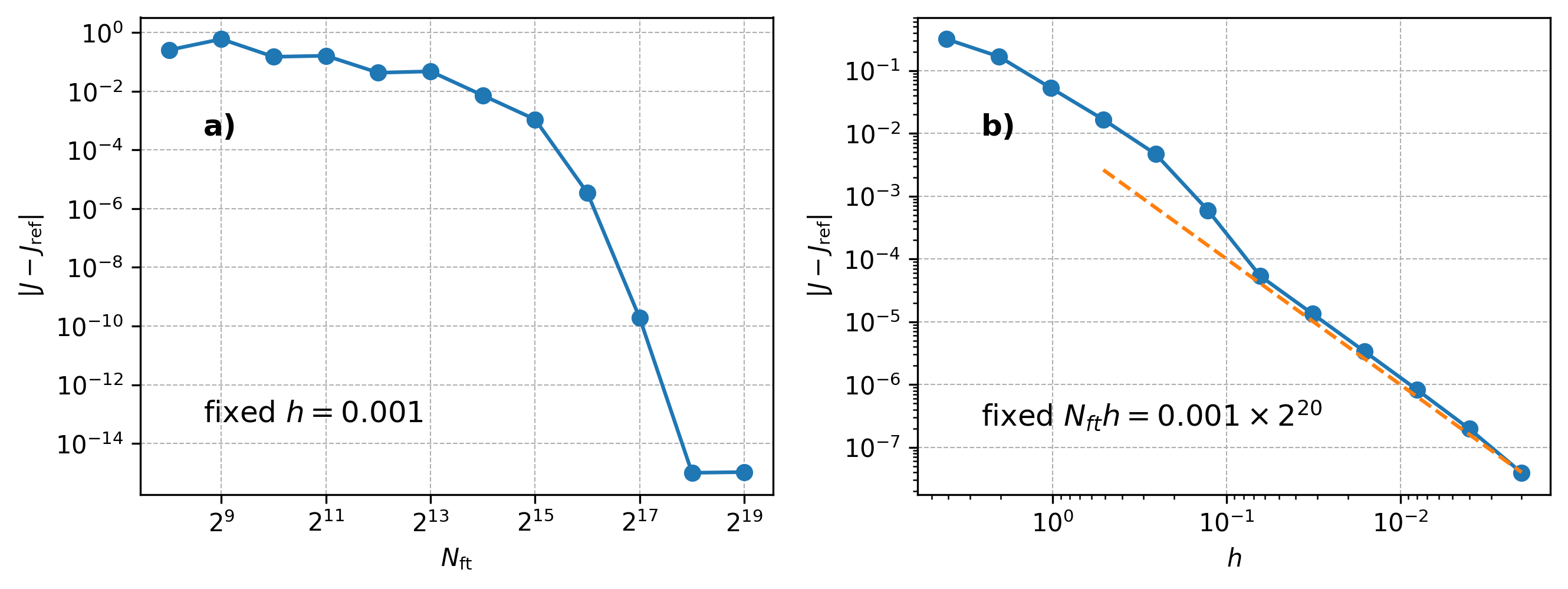
Fig. 19 Convergence results. a) Convergence of the steady state solution for fixed timestep \(h=0.001\) with \(N_{\rm ft}\) (maximal time \(t_{\rm c}\sim hN_{\rm ft}/2\)), for \(U=6\), \(V=2\), \(\beta=20\). b) Convergence of the steady state solution with the timestep \(h\), for fixed \(h N_{\rm ft}=0.001\times 2^{20}\) (fixed \(t_{\rm c}\)). In both cases, the difference \(\varepsilon=|J-J_{\rm ref}|\) of the current to a reference \(J_{\rm ref}\) is analyzed, where \(J_{\rm ref}\) corresponds to the largest grid \(N_{\rm ft}=2^{20}\) and smallest \(h=0.001\). The dashed line in b) indicates the scaling behavior \(\varepsilon\sim h^2\).

DMFT in the steady state

Synopsis

In order to benchmark the steady-state code with respect to the real-time propagation, we use a similar physical setup as in DMFT with a memory-truncated time propagation. We again consider the Synopsis Hubbard model on the Bethe lattice at half-filling, now with time-independent interaction \(U\). This requires the self-consistent solution of the equations in DMFT with a memory-truncated time propagation in the steady state. The self-energy is approximated by the second order diagram, but here we allow for two variations: (i) Self-consistent perturbation theory, where the self-energy is expanded in the fully interacting Green’s function, such that \(\mathcal{G}=G\), and (ii), iterated perturbation theory (IPT), for which \(\Sigma_U\) is expanded in the bare Green’s function of the impurity model. The latter is obtained via another Dyson equation,

\[\mathcal{G}^{-1} = i\partial_t + \mu - \Delta,\]

with the self-consistent \(\Delta\) given in DMFT with a memory-truncated time propagation.

We will solve the problem in thermal equilibrium at temperature \(T=1/\beta\) in three ways: (i) First we will use the two-time implementation with a timestep \(h_{\rm cntr}\) up to a given time \(t_{\rm max}\) (referred to as real-time or ‘cntr’ simulation in the following). Here the equilibrium state is prepared through the imaginary time branch with a given number of timesteps \(n_{\tau}\). The resulting Green’s function should be translationally invariant in time, \(G_{\rm cntr}^{R,<}(t_1,t_2)\equiv G^{R,<}(t_1-t_2)\). (ii) Thereafter, the same problem is solved using the steady-state implementation with a given Fourier domain size \(N_{\rm ft}\) and a timestep \(h_{\rm ness}\) (referred to as ‘NESS’ simulation in the following). The resulting NESS solution should match the real-time solution, \(G_{\rm cntr}^{R,<}(t_1,t_2)= G_{\rm ness}^{R,<}(t_1-t_2)\) up to numerical accuracy, so that the real-time result can be used as a benchmark for the steady state result. (iii) Finally, we will demonstrate how the steady-state result can be used to prepare an initial equilibrium solution for the real-time evolution in the memory-truncated KBE, thereby avoiding the need for the imaginary time simulation.

Details and Implementation

The relevant files for the implementation, found in nessi/examples/, are listed in the table below. For installation, see Installation.

programs/ness2_bethe_prop.cpp	Source code for real-time evolution
programs/ness2_bethe.cpp	Source code for NESS solution
programs/ness2_bethe_trunc.cpp	Memory-truncated KBE starting from NESS
utils/demo_ness2_bethe.ipynb	Jupyter notebook to run the program
utils/demo_ness2_bethe.py	Python script; same as the notebook

Implementation: Real-time simulation

The real-time benchmark ness2_bethe_prop.cpp is almost identical to the startup routine trunc_bethe_start.cpp in the example for the memory truncated KBE (DMFT with a memory-truncated time propagation), and will therefore not be discussed in detail here. The difference is that the evolution is computed at time-independent \(U\) (such that a DMFT iteration is also needed for the imaginary time branch), there is no determination of momentum-dependent Green’s functions \(G_k\), and there is an input flag ipt_flag to choose between an IPT self-energy (ipt_flag=1) and self-consistent perturbation theory (ipt_flag=0). The IPT solution just involves one more call at each timestep to solve the Synopsis Dyson equation.

Implementation: NESS simulation

The input parameters for the main program are the flag ipt_flag to choose the self-energy, the physical parameters U (interaction \(U\)), beta (inverse temperature \(\beta\)), mu (chemical potential \(\mu\)), as well as the numerical parameters Nft (number of time/frequency points) and h (timestep \(h_{\rm ness}\)). In addition, the parameters N_it (maximum number of iterations), errmax (error cutoff), and mix (linear mixing) are used to control the DMFT iteration (see below). Finally, the flag out_every allows to save the Green’s functions at every DMFT iteration. The implementation is built on the functions in the ness2 namespace, which is included at the top of the source code:

using namespace cntr;
using namespace ness2;

After reading the input from a file we allocate a herm_matrix_ness object with size=1 for the local Green’s function \(G\).

herm_matrix_ness G_ness(Nft,size);

and similar for SU_ness (\(\Sigma\)), Gweiss_ness (\(\mathcal{G}\)), and some temporary variables. Next, \(G\) is initialized with the noninteracting Green’s function.

 ness2::bethedos dos(-2,2); // bethe dos: dos(w)=sqrt(4-w**2)/(2pi)
green_equilibrium_ness(FERMION,G_ness,dos,beta,mu,h,FFT_TRAPEZ);

Because the accuracy of the initialization is not too important, we can use the faster FFT_TRAPEZ method instead of the slower FFT_ADAPTIVE. Following this, we enter a loop over at most N_it iterations for the DMFT self-consistency. At the beginning of each loop, we copy the current Green’s function into a new herm_matrix_ness object G_old. We can then compute \(\mathcal{G}\) either by copying \(\mathcal{G}=G\) (self-consistent perturbation theory), or by solving the Synopsis Dyson equation (IPT):

if(ipt_flag) dyson(Gweiss_ness,mu,ham,G_ness,h,FFT_TRAPEZ); // IPT
else  Gweiss_ness=G_ness;

Here ham is a zero matrix of dimension size=1. The computation of the self-energy is then identical to the corresponding section in the steady state example Steady-state Dyson equation: Anderson Impurity model (W_ness is a temporary herm_matrix_ness):

Bubble1_ness(W_ness, Gweiss_ness, Gweiss_ness);  // W = ii * G * G
W_ness.smul(U*U,fft_domain::time);  // W ==> W*U**2
Bubble2_ness(SU_ness, Gweiss_ness, W_ness);  // SU = ii * G * W
SU_ness.smul(-1.0, fft_domain::time);       // SU *= -1
K_ness.set_zero(fft_domain::time);          // kernel K=0
K_ness.incr(SU_ness,1.0,fft_domain::time);  // K += SU
K_ness.incr(G_ness,1.0,fft_domain::time);   // K += G (using Delta=G)

Finally, we solve the Synopsis Dyson equation, and compute the \(L_2\) norm difference to the previous iteration (stored in G_old) on the time-grid:

dyson(G_ness, mu, ham, K_ness, h, FFT_TRAPEZ); // update G_ness
err = distance_norm2(G_ness,G_old,fft_domain::time);

The convergence of the DMFT iteration is typically improved if the Green’s function at the new iteration is not taken as the updated result \(G'\), but as a linear combination \(G_{\rm new} = \alpha G' + (1-\alpha) G_{\rm old}\) (\(\alpha\) is the mixing parameter mix).

G_ness.smul(mix,fft_domain::time); // linear mixing for convergence
G_ness.incr(G_old,1.0-mix,fft_domain::time);

The DMFT iteration loop is now ended if the maximum number of iteration is reached, or if the \(L_2\) error err falls below the cutoff provided by errmax. Finally, we write all relevant Green’s functions to an HDF5 file, just as in the example Steady-state Dyson equation: Anderson Impurity model. To read the file one can again use the Python utilities provided with the ReadNESS modules.

Discussion

For illustration, we first show in Fig. 20 the convergence of the spectrum \(A(\omega)\) and the occupied density of states \(G^<(\omega)\) during the DMFT loop. In general, we observe that the linear mixing can be more relevant for the DMFT loop in the steady-state implementation than for the imaginary-time evolution within the real-time code. (In the example, we use a mixing factor \(\alpha=0.5\)). Moreover, if the time cutoff \(\sim hN_{\rm ft}\) in the simulation is not sufficient for the Dyson equation to be accurately solved, the decrease of the DMFT error with iteration would slow down around a value that is determined by the accuracy of the Dyson equation.

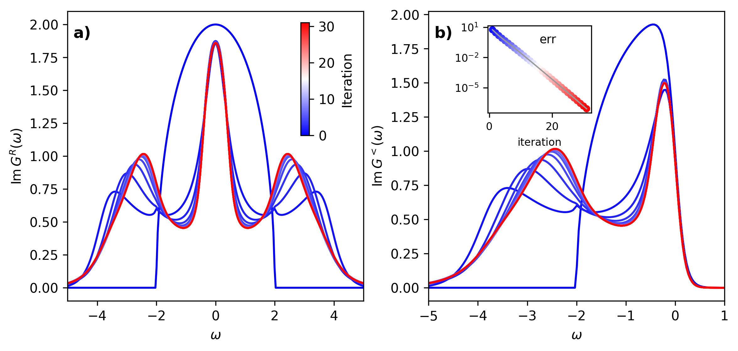
Fig. 20 DMFT convergence analysis. Steady state DMFT loop (\(U=4\), \(\beta=10\), IPT), with \(N_{\rm ft}=2^{13}\) and a timestep \(h_{\rm ness}=0.02\). (a) Convergence of spectral function \(A_{\rm iter}(\omega)\) with iteration iter=:math:0,…,30 (see color bar in a)). b) Same as (a), but for \(G^<(\omega)\). Inset in b) Convergence error \(\epsilon_{\rm iter}= |G_{\rm iter+1}-G_{\rm iter}|_2\) as function of iteration; the difference is evaluated in the time-domain.

In Fig. 21, we demonstrate that the NESS simulation and the real-time simulation converge to the same result. In equilibrium, the real-time solution results in Green’s functions which are translationally invariant in time. Their value on a given timestep \(t_1\) should therefore coincide with the NESS results,

\[X_{\rm cntr}(t_1,t_2) = X_{\rm ness}(t_1-t_2),\]

for \(X=G^{R,<},\Sigma^{R,<}\). The colored lines in Fig. 21 a) and b) show the results for the NESS simulation, while the dashed black lines correspond to the last timeslice (\(t_1=h_{\rm cntr}\cdot n_t\)) of the real-time simulation. The results indeed coincide within the line-width of the plots. Moreover, Fig. 21 c) and d) shows \(G^{R,<}(t)\) and \(\Sigma^{R,<}(t)\) on a logarithmic scale over the full time domain \(|t|<t_{\rm c}=h_{\rm ness}(N_{\rm ft}/2-1)\) of the NESS simulation. This demonstrates the decay of the functions at the boundary of the domain, which is needed for an accurate solution of the Dyson equation in the steady-state.

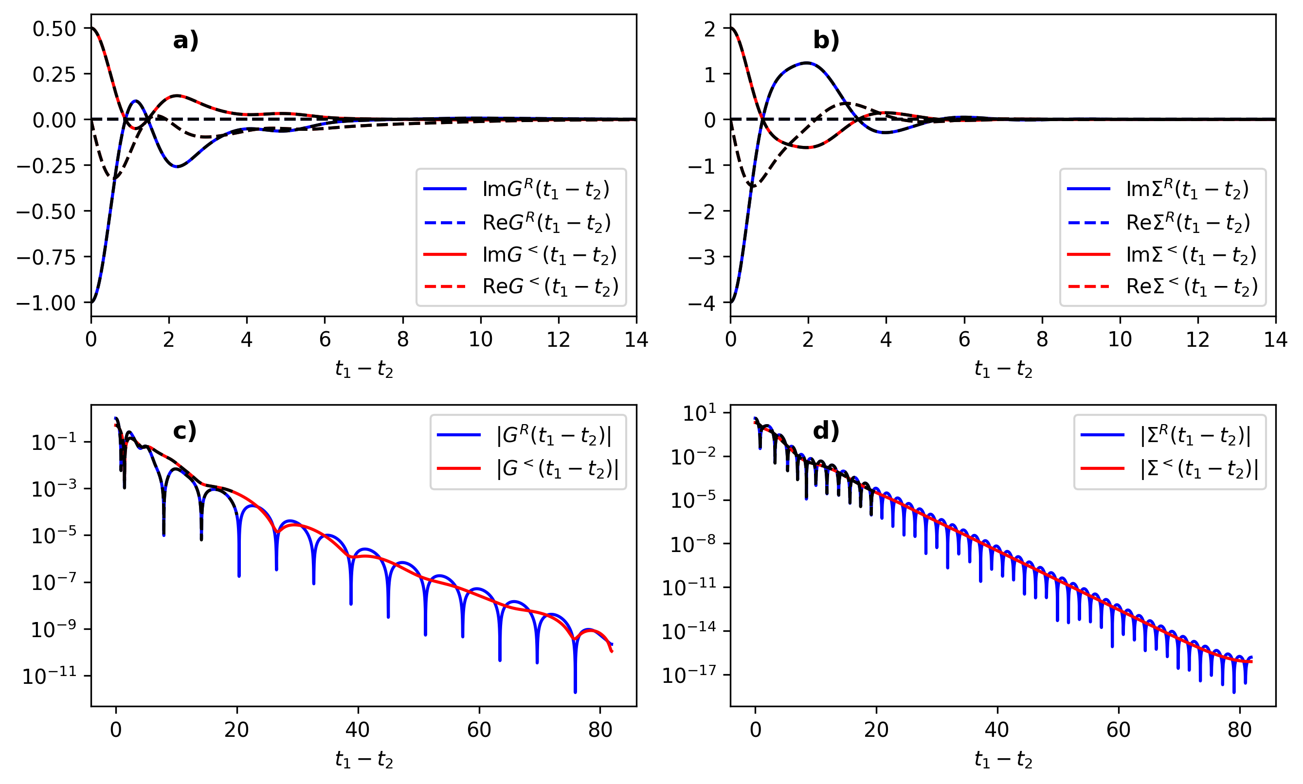
Fig. 21 Real-time comparison. Converged Green’s function \(G\) (a) and self-energy \(\Sigma\) (b) for the same parameters as in Fig. 20. Colored lines correspond to the results for the NESS simulation, while the dashed black lines, which lie on top of the colored lines, correspond to the results obtained from the last timestep of the real-time simulation (see main text). The real time simulation has been performed with \(h_{\rm cntr}=h_{\rm ness}=0.02\), nt=1000, and ntau=1000. c) and d) Same data as in panels a) and b), but on a larger time window and on a logarithmic scale.

Finally, we can quantitatively demonstrate the convergence of the NESS and real-time calculations against each other, for the same parameters (\(U=4\), \(\beta=10\), IPT). Because of the high-order accurate quadrature used in the NESSi real-time simulation, the real-time result \(G_{\rm cntr}\) with \(h_{\rm cntr}=0.02\) and ntau=1000 can be taken as an accurate benchmark. We first show the convergence of the NESS result at a fixed timestep \(h_{\rm ness}=0.02\) for increasing \(N_{\rm ft}\), corresponding to an increasing time cutoff \(t_{\rm c}\sim h_{\rm ness}N_{\rm ft}/2\). One can see that the results are converged with the cutoff for \(N_{\rm ft}\gtrsim 2^{13}\), corresponding to a cutoff \(t_{\rm c}\approx 80\). This is consistent with the exponential decay of \(G\) and \(\Sigma\). Next we perform a series of simulations with different \(N_{\rm ft}\) and fixed \(h_{\rm ness}N_{\rm ft}\), i.e., essentially varying the timestep \(h_{\rm ness}\) at fixed cutoff \(t_{\rm c}\). The convergence is analyzed in terms of the difference \(\epsilon^{R,<} = |G^{R,<}_{\rm ness}(t_1-t_2)-G^{R,<}_{\rm cntr}(t_1,t_2)|_2\) between the steady state result and the real-time benchmark \(G_{\rm cntr}\), on the largest timestep \(t_1=n_th_{\rm cntr}\) of the real-time simulation. The comparison confirms the decrease of the error like \(\mathcal{O}(h^2)\), consistent with the trapezoidal evaluation of the convolution integrals.

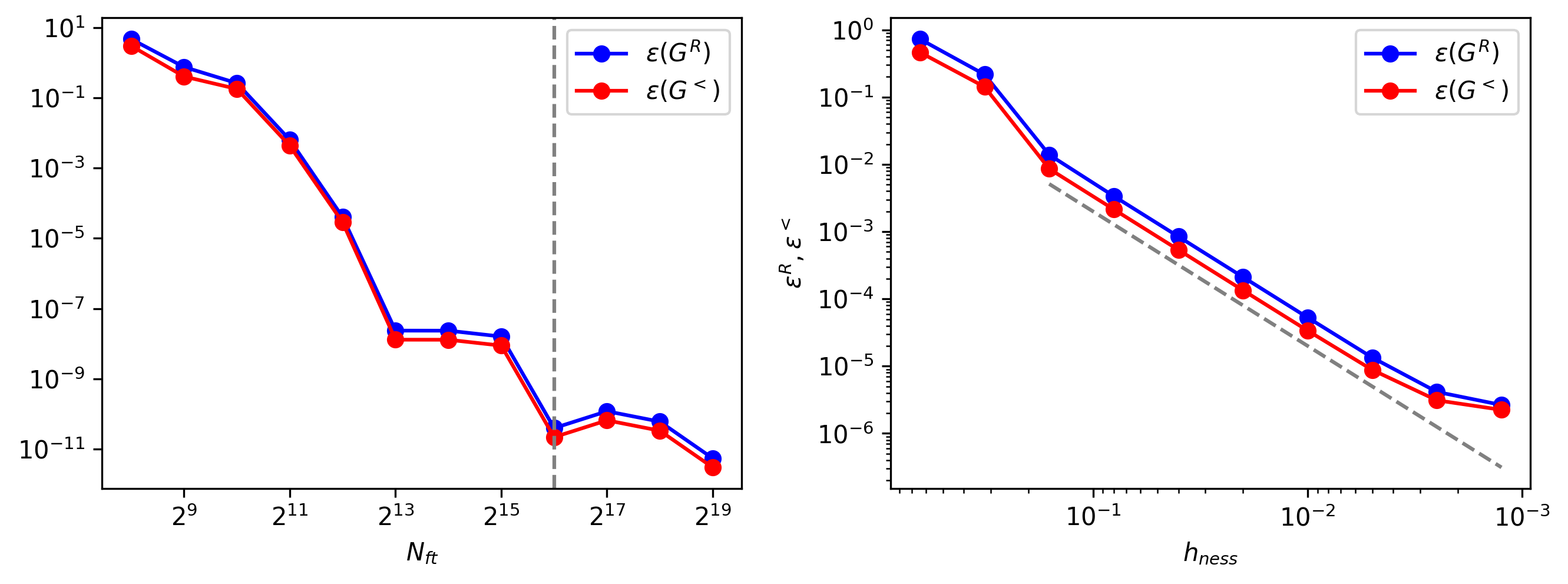
Fig. 22 NESS convergence analysis. Convergence of the NESS simulation with increasing \(N_{\rm ft}\) and decreasing \(h_{\rm ness}\) (\(U=4\), \(\beta=10\), IPT). a) Difference \(\epsilon(G^{R,<}) = |G^{R,<}_{N}-G^{R,<}_{N^*}|_2\) between a steady-state DMFT solution with domain size \(N_{\rm ft}=N\) and a reference simulation with large \(N_{\rm ft}=N^*=2^{19}\), at fixed timestep \(h_{\rm ness}=0.02\). The difference is computed on the smallest common grid. b) Difference \(\epsilon^{R,<}\equiv |G^{R,<}_{\rm ness}(t_1-t_2)-G^{R,<}_{\rm cntr}(t_1,t_2)|_2\) between the steady state result and the real-time benchmark \(G_{\rm cntr}\), as function of \(h_{\rm ness}\) (see main text). Results are obtained for fixed \(N_{\rm ft}\times h_{\rm ness}=2^{16}\times 0.02\); corresponding to a cutoff \(t_{\rm c}\approx 650\) well beyond the convergence threshold found in a). The dashed line in (b) indicates an error scaling \(\epsilon \sim h^2\).

Interface with truncated KBE

Because both the memory-truncated and the NESS Green’s functions are entirely defined in terms of their real-time components \(G^R\) and \(G^<\), one can straightforwardly exchange data between the two objects. Here we provide an example that illustrates how a NESS simulation can be used to initialize the time evolution with the truncated KBE. This circumvents the initialization via the imaginary time propagation, as in the startup routine of the example in DMFT with a memory-truncated time propagation. In detail, we will initialize memory-truncated Green’s functions and self-energies for the Hubbard model on a Bethe lattice using the result of the steady-state simulation in ness2_bethe.x, and then use the truncated KBE to further propagate the solution in time. While the expected result should simply maintain the time-translationally invariant solution for all times, this is still a numerically nontrivial test which can be used straightforwardly to access the accuracy of the approach.

Running the test is also part of demo_ness2_bethe.ipynb. We first use the NESS simulation with ness2_bethe.x to prepare a steady-state equilibrium solution with a given timestep \(h_{\rm ness}\) and domain size \(N_{\rm ft}\). The output file of the NESS simulation is then read by the executable ness2_bethe_trunc.x, to perform the truncated KBE simulation. Because the numerical error in the NESS simulation decreases with the timestep only like \(\mathcal{O}(h^2)\), in contrast to the higher order accurate real-time KBE implementation, it can be beneficial to perform the NESS simulation with a smaller timestep than the one used in the truncated evolution. We will set \(h_{\rm cntr}=d\cdot h_{\rm ness}\), with an integer factor \(d\).

The truncated simulation thus takes as input the parameters downsampling (the factor \(d\)), tc (memory cutoff in the KBE simulation), tmax (the number of timesteps over which the KBE is propagated), out_every (frequency at which timeslices of the KBE are written to file), and CorrectorSteps (number of DMFT iterations at each timestep, see explanation in Details and Implementation). Further parameters (\(U\), \(\beta\), \(h_{\rm ness}\), \(N_{\rm ft}\), and the ipt_flag) are read, together with the Green’s functions, from the HDF5 file which is written as output of the NESS simulation.

After reading the input, the main step is the initialization of the memory-truncated functions, which we explain exemplarily for the Green’s function. (All routines use namespaces ness2 and cntr.) First we allocate the memory truncated function with a cutoff tc and orbital dimension size=1,

herm_matrix_moving<double> Gcntr(tc,1,FERMION);

We then read the NESS Green’s functions from the HDF5 output of the NESS simulation (with name ness_filename), where it is stored under a group G:

herm_matrix_ness Gness;
Gness.read_from_hdf5(ness_filename,"G");

The object Gness is thereby also resized to the correct dimension Nft. Since the real-time evolution will be run on a grid that is coarser by a factor \(d\), we must downsample the steady-state Green’s function:

herm_matrix_ness Gness1;
Gness1=downsample(Gness,downsampling);

This will automatically resize Gness1 to the correct dimension Nft1, where Nft1=Nft/downsampling. In the time-domain, downsampling simply copies every \(d\)-th value of Gness (on the fine grid) to Gness1 (coarse grid). In turn, the frequency grid is restricted to the lowest frequencies {-Nft1/2, ..., Nft1/2-1}. The routine therefore requires Nft to be an integer multiple of \(d\), and Nft1 to be a multiple of \(2\). Here we choose both Nft and \(d\) to be a power of \(2\). Finally, the memory truncated Green’s function is initialized using

ness2cntr(Gcntr, Gness1);

Here ness2cntr will initialize \(G_{\rm cntr}\) such that

\[G_{\rm cntr}^{<,R}(t_1,t_2)=G^{<,R}_{\rm ness}(t_1-t_2)\]

is translationally invariant in time in the full domain \(\mathcal{M}[G]\). The cutoff tc of \(G_{\rm cntr}\) should be smaller or equal to the maximum number of timesteps in Gness1, which is Nft1/2-1; otherwise part of \(G_{\rm cntr}\) would be left zero. The initialization is repeated for the self-energy and for \(\mathcal{G}\), which are both stored in the NESS output file.

After this point, the truncated time evolution in ness2_bethe_trunc.x is identical to the example of Details and Implementation, where the truncated Green’s functions are initialized from a full real-time simulation. Selected timeslices t of the KBE simulation will be stored in the HDF5 output file under a group with key t[t]/G. Alternatively to writing the slices directly, as in the example trunc_bethe above, we can use the reverse data exchange cntr2ness to initialize a herm_matrix_ness from the real-time Green’s function, and store the latter:

void write_slice(hid_t fl_id,int t,herm_mat_moving<double> &Gcntr){
  // fl_id is a handle to an open and writable HDF5 file
  [...] // create herm_matrix_ness Gness with Nft/2-1>=G.tc_
  cntr2ness(Gness,Gcntr); // read last timestep of G into Gness
  // write Gness to new group t[t]/G in file fl_id:
  hid_t sub_group_id = create_group(file_id,"t"+std::to_string(t));
  Gness.write_to_hdf5(sub_group_id, "G");
  close_group(sub_group_id);
}

Exemplary results are shown in Fig. 23. We perform the test for similar parameters as in the example in Discussion, using a self-consistent perturbation theory for \(U=1\) and \(\beta=2\). Note that this high temperature rather corresponds to the order of magnitude of the final thermalised temperature in the previous example, rather than to the initial temperature before the quench. Lower temperatures typically require a longer memory cutoff, because a sharp Fermi edge in the distribution function \(G^<(\omega)\) implies a slower decay of \(G^<(t)\). We also observe that the IPT simulation is less stable under a long-time evolution, which may be related to its non-conserving nature.

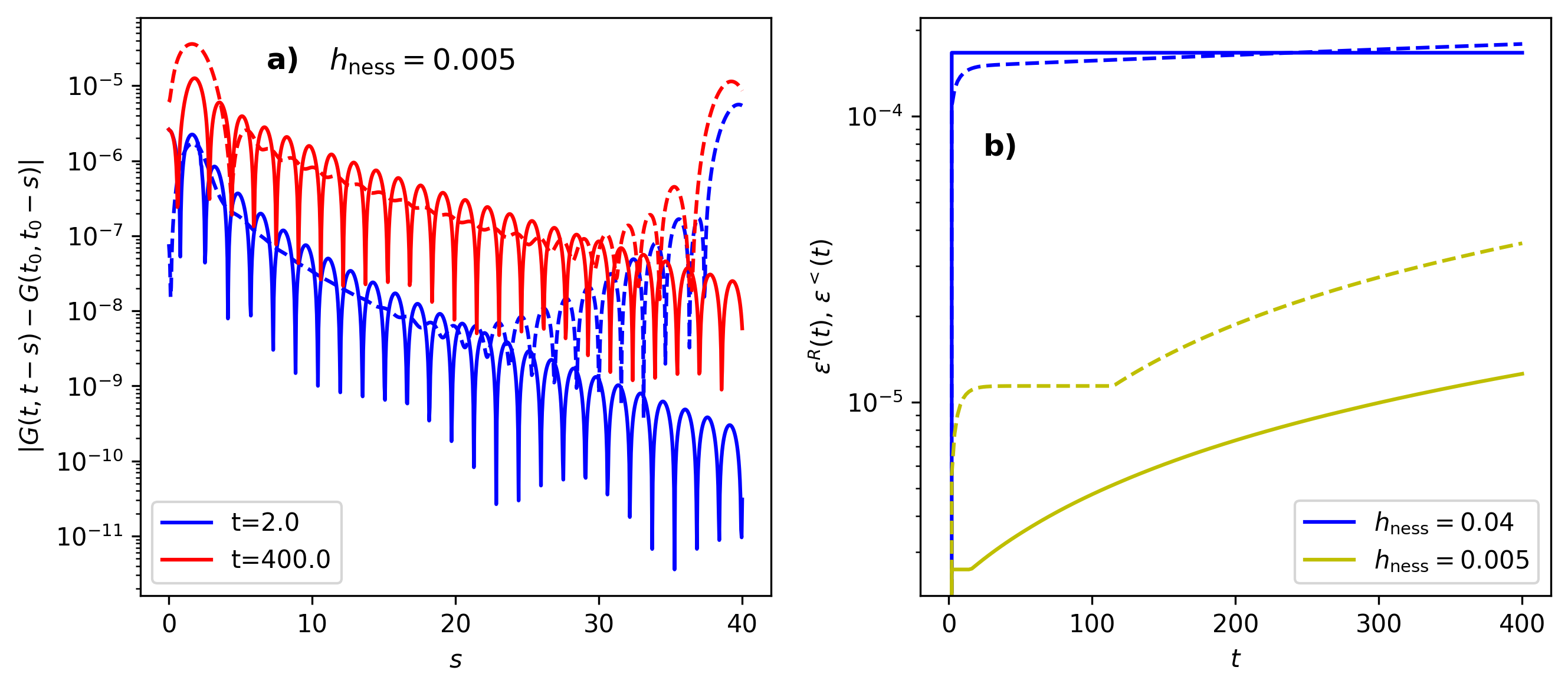
Fig. 23 Memory truncated time-evolution of an equilibrium state initialized with a NESS simulation. Self-consistent perturbation theory, \(U=1\), \(\beta=2\). The truncated KBE evolution is performed with \(h_{\rm cntr}=0.04\) and a cutoff tc=1000, and the initial NESS simulation uses \(h_{\rm ness}=0.005\). a) Difference \(\epsilon^{R,<}(t,s)=|G_{\rm cntr}^{R,<}(t,t-s)-G_{\rm cntr}^{R,<}(t_0,t_0-s)|\) between the Green’s functions on timeslice \(t\) and the first timeslice \(t_0=0\). Full (dashed) lines show \(\epsilon^R\) (\(\epsilon^<\)). b) Maximum difference \(\epsilon^{R,<}(t)=\text{max}_s (\epsilon^{R,<}(t,s))\) as function of \(t\), for different \(h_{\rm ness}\).

Fig. 23 a) shows the comparison of the real-time result \(G_{\rm cntr}^{R,<}(t,t-s)\) to the initial NESS Green’s function \(G_{\rm ness}^{R,<}(s)\), which match by construction on the initial timeslice \(t=0\). The two timeslices \(t=2\) and \(t=400\) correspond to \(50\) and \(10000\) timesteps \(h_{\rm cntr}=0.04\), respectively. One can see that very early a difference is built up in the lesser component at large relative times \(s\), which is related to the finite cutoff \(t_c\) in the memory-truncated evolution. Thereafter, the difference \(|G_{\rm cntr}^{R,<}(t,t-s)-G_{\rm ness}^{R,<}(s)|\) grows slowly with time due to a regular linear error accumulation (but remains small on the absolute scale). In Fig. 23 b) we analyze the maximum difference

\[\epsilon^{R,<}(t)=\text{max}_s\left(|G_{\rm cntr}^{R,<}(t,t-s)-G_{\rm ness}^{R,<}(s)|\right)\]

over a timeslice \(t\) as function of \(t\). If the NESS simulation is performed with the same timestep as the real-time simulation, the NESS simulation is less accurate and therefore slightly inconsistent with a translationally invariant real-time solution (see the results for \(h_{\rm ness}=h_{\rm cntr}=0.04\) in Fig. 23 b). The time-evolution then leads to the buildup of a finite difference \(\epsilon^{R,<}(t)\) over few timesteps, so that the linear error accumulation starts from a higher level. This initial error buildup can be simply reduced by performing the NESS simulation with a smaller timestep (see the results for \(h_{\rm ness}=0.005\) in Fig. 23 b). Since the numerical cost of the NESS simulation scales only with \(\mathcal{O}(N_{\rm ft}\log N_{\rm ft})\) due to the use of FFT, the preparation of the equilibrium state via the NESS simulation is still cheaper than the preparation via a full real-time evolution.