Diagram Utilities

The basic building blocks of Feynman diagrams are particle-hole bubbles and particle-particle bubbles, such as:

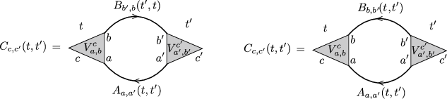
The figure shows a typical particle-hole (left) and particle-particle (right) bubble, where \(V^c_{ab}\) is an interaction vertex depending on three orbital indices, and \(A\) and \(B\) are Green’s functions. The diagrams above correspond to the following algebraic expressions:

(3)\[\text{particle-hole bubble:}\,\,\,C_{c,c'}(t,t') = \sum_{a,a'} \sum_{b,b'} V^c_{a,b} \Big[ iA_{a,a'}(t,t') B_{b',b}(t',t) \Big] V^{c'}_{a',b'},\]

(4)\[\text{particle-particle bubble:}\,\,\,C_{c,c'}(t,t') = \sum_{a,a'} \sum_{b,b'} V^c_{a,b} \Big[ i A_{a,a'}(t,t') B_{b,b'}(t,t') \Big] V^{c'}_{a',b'}.\]

Note on hermitian conjugation: The complex \(i\) factor has been inserted for convenience. With this definition, the hermitian conjugate \(C^\ddagger\) of \(C\) is obtained simply by replacing A and B by their hermitian conjugates, and \(V^c_{a,b}\) by its element-wise complex conjugate. In particular, if \(V\) is real and A and B are hermitian symmetric, then also C is hermitian symmetric (as a matrix-valued Green’s function; its individual components are not hermitian, but \((C_{1,2})^\ddagger = C_{2,1}\)).

The basic building blocks are therefore products of the type \(C(t,t')=iA_{a,a'}(t,t') B_{b',b}(t',t)\) and \(C(t,t')=iA_{a,a'}(t,t') B_{b,b'}(t,t')\), where \(t,t'\) are arbitrary times on the contour. To evaluate those products, one uses Langreth rules. For example:

(5)\[C(t,t')=iA(t,t')B(t',t) \,\,\,\Rightarrow\,\,\, C^<(t,t')=iA^<(t,t')B^>(t',t)\]

We provide two basic functions that allow to compute particle-particle and particle-hole Bubbles on a given timestep:

cntr::Bubble1(int tstp, GG &C,int c1,int c2,GG &A,GG &Acc,int a1,int a2,GG &B,GG &Bcc,int b1,int b2)	\(C_{c1,c2}(t,t')=i A_{a1,a2}(t,t') B_{b2,b1}(t',t)\) is calculated on timestep tstp of C for given two-time objects A,B with matrix indices a1, a2 and b1, b2, respectively. output: object C with matrix indices c1, c2
cntr::Bubble2(int tstp, GG &C,int c1,int c2,GG &A,GG &Acc,int a1,int a2,GG &B,GG &Bcc,int b1,int b2)	\(C_{c1,c2}(t,t')=i A_{a1,a2}(t,t') B_{b1,b2}(t,t')\) is calculated on timestep tstp of C for given two-time objects A,B with matrix indices a1, a2 and b1, b2, respectively. output: object C with matrix indices c1, c2

• C, A, Acc, B, Bcc can be of type cntr::herm_matrix or cntr::herm_matrix_timestep

• For X``=``A or B: Xcc contains the hermitian conjugate \(X^\ddagger\) of \(X\). If the argument Xcc is omitted, it is assumed that X is hermitian, \(X=X^\ddagger\).

• If the index pairs (c1,c2), (a1,a2), or (b1,b2) are omitted, they are assumed to be (0,0)

• The following size requirements apply:

  • For all X = C, A, Acc, B, Bcc: X.tstp()==tstp required if X is of type herm_matrix_timestep, and X.nt()>=tstp required if X is of type herm_matrix

  • A.size1()>=a1,a2 required, analogous for C, A, Acc, B, Bcc

  • X.ntau() must be equal for all X = C, A, Acc, B, Bcc

• From (5) one can see that in general A and B must be known outside the hermitian domain in order to compute C in the hermitian domain, which is why the hermitian conjugates \(A^\ddagger\) and \(B^\ddagger\) must be provided as arguments.

Example 1:

The following example calculates the second-order self-energy for a general time-dependent interaction \(U(t)\) out of a scalar local Green’s function, \(\Sigma(t,t') = U(t) G(t,t') G(t',t) U(t') G(t,t')\). The diagram is factorised in a particle-hole bubble \(\chi\) and a particle-particle bubble:

\[\Sigma(t,t') = -i W(t,t') G(t,t'), \,\,\,\, W(t,t')=U(t) \chi(t,t') U(t'), \,\,\,\,\, \chi(t,t') = iG(t,t') G(t',t).\]

int nt=10;
int ntau=100;
int size1=1;
GREEN G(nt,ntau,size1,FERMION);
GREEN Sigma(nt,ntau,size1,FERMION);
CFUNC U(nt,size1);
// ...
// ... do something to set G and U
// ...
// compute Sigma on all timesteps:
for(int tstp=-1;tstp<=nt;tstp++){
    GREEN_TSTP tW(tstp,ntau,size1,BOSON); // used as temporary variable; Note that a bubble of two Fermion GF is bosonic
    cntr::Bubble1(tstp,W,G,G); // W(t,t') is set to chi=ii*G(t,t')G(t',t);
    // Note: Because G is scalar and have hermitian symmetry, many arguments can be replaced by default. The above extends to
    // cntr::Bubble1(tstp,W,0,0,G,G,0,0,G,G,0,0,);
    W.left_multiply(tstp,U);
    W.right_multiply(tstp,U); // now W is set to W(t,t')=U(t)chi(t,t')U(t')
    cntr::Bubble2(tstp,Sigma,G,W); // Sigma(t,t') is set to Sigma=ii*G(t,t')W(t',t);
    // Note that by construction, W is hermitian, see above
    Sigma.smul(tstp,-1.0); // the final -1 sign.
}

Example 2:

Evaluation of the diagrams (3) and (4), where A and B are two-dimensional, C is one-dimensional, and V is a corresponding contraction. The contraction over internal indices is done by an explicit four-dimensional summation.

int nt=10;
int ntau=100;
int size1=2;
int sizec=1;
GREEN A(nt,ntau,size1,FERMION);
GREEN B(nt,ntau,size1,FERMION);
GREEN CPH(nt,ntau,sizec,BOSON);
GREEN CPP(nt,ntau,sizec,BOSON);
// ...
// compute particle-hole bubble (CPH) and particle-particle bubble (CPP) on all timesteps:
for(int tstp=-1;tstp<=nt;tstp++){
    GREEN_TSTP ctmp(tstp,ntau,1,BOSON); // temporary
    CPH.set_timestep_zero(tstp);
    CPP.set_timestep_zero(tstp);
    for(int a1=0;a1<size1;a1++){
     for(int a2=0;a2<size1;a2++){
      for(int b1=0;b1<size1;b1++){
       for(int b2=0;b2<size1;b2++){
            double v1=get_vertex(a1,b1); // supposed to return V_{a1,b1}
            double v2=get_vertex(a2,b2); // supposed to return V_{a2,b2}
            cntr::Bubble1(ctmp,0,0,A,A,a1,a2,B,B,b1,b2); // Note the order of the arguments b1,b2!
            CPH.incr_timestep(tstp,ctmp,v1*v2);
            cntr::Bubble2(ctmp,0,0,A,A,a1,a2,B,B,b1,b2);
            CPP.incr_timestep(tstp,ctmp,v1*v2);
       }
      }
     }
    }
}