Green Functions
Overview
class |
|
This class contains the data structures for representing two-time contour functions \(C(t,t')\) on the equidistantly discretized time-contour \(\mathcal{C}\) with points \(\{i\Delta t: i=0,1,2,...,{\tt nt}\}\) along the real time branch, and \(\{i\Delta\tau,i=0,1,...,{\tt ntau}\}\) along the imaginary branch. The Green’s functions are defined by the following parameters:
T(template parameter): Precision, usually set todouble; we use the global definition#define GREEN cntr::herm_matrix<double>ntandntau(integer): number of discretization points on the real and imaginary time axis.size1(integer): orbital dimension. Each element \(C(t,t')\) is a square matrix of dimensionsize1\(\times\)size1.sig(integer): Takes the valuesFERMION(defined as-1) orBOSON(+1).
herm_matrix stores the following Keldysh components on the equidistantly discretized Keldysh contour with time discretization \(\Delta t\) and \(\Delta \tau\) on the real and imaginary time, respectively (The real-time domain of a herm_matrix object is illustrated in the Figure):
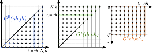
Matsubara component \(C^\mathrm{M}(i\Delta \tau)\) for
i=0,...,ntau,retarded component \(C^\mathrm{R}(i\Delta t,j\Delta t)\) for
i=0,...,nt,j=0,...,i,lesser component \(C^<(i\Delta t,j\Delta t)\) for
j=0,...,nt,i=0,...,j,left-mixing component \(C^\rceil(i\Delta t,j\Delta \tau)\) for
i=0,...,nt,j=0,...,ntau.
If nt = -1, only the Matsubara component is stored.
Size arguments of herm_matrix are returned by the following read-only member functions:
GREEN G;
cout << "The object G of type herm_matrix has the following dimensions:" << endl;
cout << "nt= " << G.nt() << endl;
cout << "ntau= " << G.ntau() << endl;
cout << "size1= " << G.size1() << endl;
cout << "sig= " << G.sig() << endl;
Hermitian symmetry and conjugate:
In the following, we call the components mentioned above the hermitian domain of a two-time contour function.
The Hermitian conjugate \(C^\ddagger\) of a Green’s function \(C\) is defined (\(\xi=\) +1 and -1 for BOSON and FERMION, respectively):
\([C^\ddagger]^\mathrm{R}(t,t^\prime) = \left( C^\mathrm{A}(t^\prime,t)\right)^\dagger \ ,\)
\([C^\ddagger]^\gtrless(t,t^\prime) = -\left( C^\gtrless(t^\prime,t) \right)^\dagger \ ,\)
\([C^\ddagger]^{\rceil}(t,\tau) = - \xi \left( C^\lceil(\beta-\tau,t) \right)^\dagger \ ,\)
\([C^\ddagger]^{\mathrm{M}}(\tau) =\left( C^{\mathrm{M}}(\tau) \right)^\dagger \ .\)
Apparently, \(C=(C^\ddagger)^\ddagger\).
Hence, if a Green’s function has hermitian symmetry (\(C=C^\ddagger\)), it is sufficient to use one object of type herm_matrix and store the hermitian domain. If a Green’s function is not hermitian, one must store the hermitian domain of \(C\) and of \(C^\ddagger\) in two separate herm_matrix variables.
For a summary of all member functions, see Summary: Member Functions of herm_matrix and herm_matrix_timestep[_view]. The following paragraphs give detailed explanations of some functionalities.
Constructors
|
Default constructor, does not allocate memory, sets |
|
Allocate memory, and sets all entries to |
|
Equivalent to |
Accessing individual elements
The following routines allow to read/write the elements of a contour function \(C(t,t')\) stored as herm_matrix at individual time arguments from/to another variable M. The latter can be either a scalar of type std::complex<T>, or a complex square matrix defined in Eigen (see Scalar and matrix types).
Member functions of herm_matrix:
Member functions of herm_matrix allow to read/write elements of \(C\) in the hermitian domain. To read elements of \(C\) outside the hermitian domain (which are reconstructed from \(C\) and \(C^\ddagger\)), one can use the non-member element access functions defined later.
The following member functions set components of a contour function \(C\) in the hermitian domain from M:
|
\(C^<(i\Delta t,j\Delta t)\) is set to |
required: |
|
\(C^R(j\Delta t,i\Delta t)\) is set to |
required: |
|
\(C^{\rceil}(i\Delta t,j\Delta \tau)\) is set to |
required: |
|
\(C^M(i\Delta \tau)\) is set to |
required: |
If
C.size1()>1,Mmust be a complex eigen matrix (cdmatrixfor double precision)If
C.size1()==1,Mcan be a scalar (cdouble) or a matrixIf
Mis a Matrix, it must be a square matrix of dimensionsize1
The following member functions read components of a contour function \(C\) in the hermitian domain to M:
|
|
required: |
|
|
required: |
|
|
required: |
|
|
required: |
If
Mis a matrix, it is resized to a square matrix of dimensionC.size1()If
Mis a scalar, only the (0,0) entry of \(C(t,t')\) is read.
Remark: Member functions set_les and set_ret can return also values outside the hermitian domain (assuming that \(C\) has hermitian symmetry), but this functionality is no longer supported. Similarly, there are non-supported member functions like get_gtr(...) which return other Keldysh components. Use instead the general access functions described in the next paragraph.
General element access:
The following functions read components of a contour function \(C\) to M:
|
|
required: |
|
|
required: |
|
|
required: |
|
|
required: |
|
|
required: |
|
|
required: |
CandCccare (size-matched) arguments of typeherm_matrixwhich store the hermitian domain of \(C\) and its hermitian conjugate \(C^\ddagger\).If the argument
Cccis omitted, hermitian symmetry \(C=C^\ddagger\) is assumed.If
Mis a matrix, it is resized to a square matrix of dimensionC.size1().Mmay always be a scalar; in this case only the (0,0) entry of \(C(t,t')\) is read.
Note
All set_XXX and get_XXX element access functions are not optimised for massive read/write operations. (In particular, set_XXX and get_XXX are not used inside the numerically costly tasks like the solution of integral equations). Mostly, data are anyway read and written timestep-wise (see Timeslices).
Density matrix
The equal-time elements of Green’s functions contain expectation values of physical observables. If \(C_{ab}(t,t') = -i \langle T_\mathcal{C} \hat A_a(t)\hat B_b(t')\rangle\) is the contour ordered expectation value of two operators \(\hat A\) and \(\hat B\) (such as creation and annihilation operators with orbital indices a and b) then the time-dependent expectation value \(\rho_{ab}(t) = \langle B_{b} A_{a} \rangle_t\) is given by (\(\xi\) is the BOSON/FERMION sign):
We therefore define the Density matrix of a two-time Green’s function on the discretized contour at timestep tstp as:
The following member function of a cntr::herm_matrix<T> object C writes the Density matrix to an object M:
|
|
tstp <= C.nt()required.If
C.size1()>1,Mmust be a complex eigen matrix (cdmatrixfor double precision)If
C.size1()==1,Mcan be a scalar (cdouble) or a matrixIf
Mis a matrix, it is resized to a square matrix of dimensionC.size1().
File I/O
Reading/writing to text files
The member functions print_to_file and read_to_file of a herm_matrix implement text-file access, as apparent by example:
int nt=10;
int ntau=10;
int size1=2;
int sig=FERMION;
GREEN A(nt,ntau,size1,sig);
// ... set elements of  A ...

//WRITE:
// create a file filename.txt and store the data of A:
A.print_to_file("filename.txt");

// READ
GREEN B;
// if the file "filename.txt" has been written previously with print_to_file ,
// the parameters (nt,ntau,size1,sig) and the data of B are modified
// according to the information in the file:
B.read_from_file("filename.txt");
// now B is resized to B.nt()=10, B.ntau()=10,B.size1()=2,B.sig()=FERMION, and the data of B match the data of A.
The file format is rather explicit (and storage intensive):
First line:
# nt ntau size1 sigThe following lines list the Matsubara component in the format:
mat: i Re_C^mat(i)_{0,0} Im_C^mat(i)_{0,0} ... Re_C^mat(i)_{size1,size1} Im_C^mat(i)_{size1,size1}If
nt>-1, the following lines list the other components in the format:XXX: i j Re_C^XXX(i,j)_{0,0} Im_C^XXX(i,j)_{0,0} ... Re_C^XXX(i,j)_{size1,size1} Im_C^XXX(i,j)_{size1,size1}whereXXXisretfor \(C^R\),lesfor \(C^<\),tvfor \(C^{\rceil}\), andi,jloop through the corresponding time arguments of the hermitian domain.
Note
Writing to text files is supposed as a quick way to generate human-readible data. For compressed storage, one should use the HDF5 format below.
Reading/writing to hdf5 files
The HDF5 format, as well as some scripts to interpret the hdf5 files are discussed in a separate section HDF5 Usage below.